Lately, my son has been very curious about words, so I have decided that it is a great time for us to practice letters. One way we practice is with flash cards. I like this method since it is easy to get in a few practice letters between other activities. The problem I am facing is how to choose which letters we practice. Ideally, I want to cover all letters over time, but focus on those he doesn’t know and adapt as he learns them.

…enter the adversarial multi-armed bandit!

Given an array of choices that can be repeated, bandit strategies seek to maximize rewards by learning from past choices. I can frame my problem in this way by seeing each letter as a choice and my son’s response as an outcome. Since I want to optimize towards letters he has not yet learned, I will “reward” the model when a letter is chosen that he does not recognize. An issue with this approach is that when my son responds by learning a new letter, my model will have a hard time un-learning to choose that letter. In fact, I expect a diminishing return as I repeat letters and he becomes more likely to recognize them. In this sense, my son’s responses are “adversarial”.

Besides being a great band name, an adversarial multi-armed bandit is designed to optimize choices over time, even when the mean reward for each choice is non-stationary. It does this by balancing randomness against learned probabilities that decay over time.

The algorithm I have chosen is Exp3, which is short for Exponential-weight algorithm for Exploration and Exploitation. In terms of my situation:

• Exploration - randomly choosing letters to determine my son’s knowledge of the alphabet (also has the up-side of occasionally reinforcing letters he already knows)
• Exploitation - preferring letters that he has not done well on in the past

Let’s make some code! Here are my functions in R for assigning weights to letters and deriving probabilities from those weights.

### Utility Functions ###
# update the weight given to a choice, based on the reward for a trial
updateWeight <- function(weight, probs, choice, reward, g=0.0){
  estimatedReward = reward / probs[choice]
  weight * exp(estimatedReward * g / length(probs))
}

# create a probability vector from the vector of weights
getProbabilities <- function(weights, g=0.0){
  (1.0 - g) * (weights / sum(weights)) + (g / length(weights))
}

Now to set up the problem and initialize my parameters. The g (gamma) parameter is a tuning parameter for Exp3 that provides theoretical limits to regret (the difference between optimal performance and actual performance). It does this by controlling the balance between exploration and exploitation as described above.

# choices = alphabet
choices = unlist(strsplit('ABCDEFGHIJKLMNOPQRSTUVWXYZ', ''))
# upper bound on cumulative reward over convergence time horizon (assuming 1,000 trials)
upperBoundEstimate = 1000
# set gamma parameter
g = min(1, sqrt((length(choices) * log(length(choices))) / ((exp(1) - 1) * upperBoundEstimate)))
# initialize weights
choiceWeights = rep(1, length(choices))
choiceProbs = getProbabilities(choiceWeights, g)

Each time I get new data, I can do the following to update my model. Note that I have coded my son’s responses in the “Recognized” column, with 1 == recognized and 0 == not recognized. I can also assign scores in between, for example: 0.5 if he recognized the letter after being given a hint as to the sound it makes.

### load data ###
trials = read.csv('AlphabetTrials.csv')
# names(trials) -> c('Letter', 'Recognized')
numTrials = nrow(trials)

### loop through trials ###
for( i in 1:numTrials ){
  # choice is index of letter in alphabet
  choice = which(choices == trials$Letter[i])
  # reward == finding a letter that is not recognized
  reward = 1 - trials$Recognized[i]
  # update weights
  choiceWeights[choice] = updateWeight(choiceWeights, choiceProbs, choice, reward, g)
  # get associated probabilities
  choiceProbs = getProbabilities(choiceWeights, g)
}

When I want to choose another set of 5 letters to practice, I can simply run:

# get next 5 choices for future trials
next5Choices = sample(choices,5,prob=choiceProbs)
# c('U', 'A', 'Z', 'Y', 'F')

This samples from the model’s probability distribution of letters. After 72 trials, my distribution looks like this:

# formatting
par(lty=0)
par(mar=c(3,4,1,1))
# final probabilities
barplot(choiceProbs, names.arg = choices, col=myHeatColorRamp(5)[ceiling(choiceProbs*100)-2], ylab='Probability',space=0)
par(lty='solid')
# grid lines
abline(h=seq(0.01, 0.06, 0.01), col=rgb(1, 1, 1, alpha=0.3), lwd=2,lty='solid')

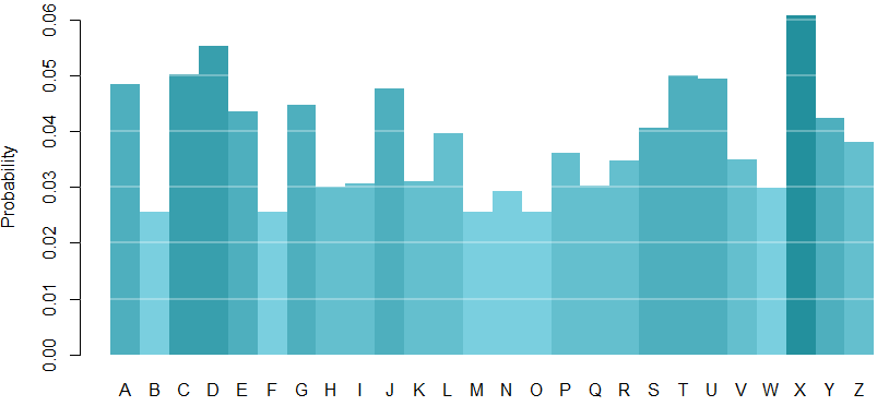It looks like ‘X’, ‘D’, and ‘C’ are letters we may need to practice.

I have really been enjoying this method and it seems to work well, but how do I know that it is better than other methods? Without knowing what he would answer for each letter in any given round, there are some ways I can estimate my effectiveness. Based on the results I have seen so far, I would estimate that my son had knowledge of about 30% of letters before we began and 48% now. Assuming that he has progressed linearly, I can compare the actual cumulative reward (ability to find letters he didn’t know yet) to the expected cumulative reward from a purely random method.

# optimal cumulative reward
plot(1:numTrials, 1:numTrials, type='l', col=myColors[11], lwd=3, bty='n',xlab='Trials', ylab='Cumulative Reward')
# grid lines
abline(h=seq(0,100,20), col=rgb(0.6, 0.6, 0.6, alpha=0.3), lty='solid')
abline(v=seq(0,100,20), col=rgb(0.6, 0.6, 0.6, alpha=0.3), lty='solid')
# expected random reward, assuming linear decline from 0.7 avg reward to 0.52
expectedRandom = cumsum((1:numTrials / numTrials)*0.52 + (1-(1:numTrials / numTrials))*0.7)
# difference between actual and expected
polygon(c(1:numTrials,rev(1:numTrials)), c(cumsum(1 - trials$Recognized),rev(expectedRandom)),col=myColors[1])
lines(1:numTrials, expectedRandom, lwd=3, col=myColors[4])
# actual reward
lines(1:numTrials, cumsum(1 - trials$Recognized), lwd=3, col=myColors[3])
# labels
text(46, 54, labels='Optimal', cex=1.2, col=myColors[11])
text(53, 43, labels='Actual', cex=1.2, col=myColors[3])
text(67, 36, labels='Random', cex=1.2, col=myColors[4])

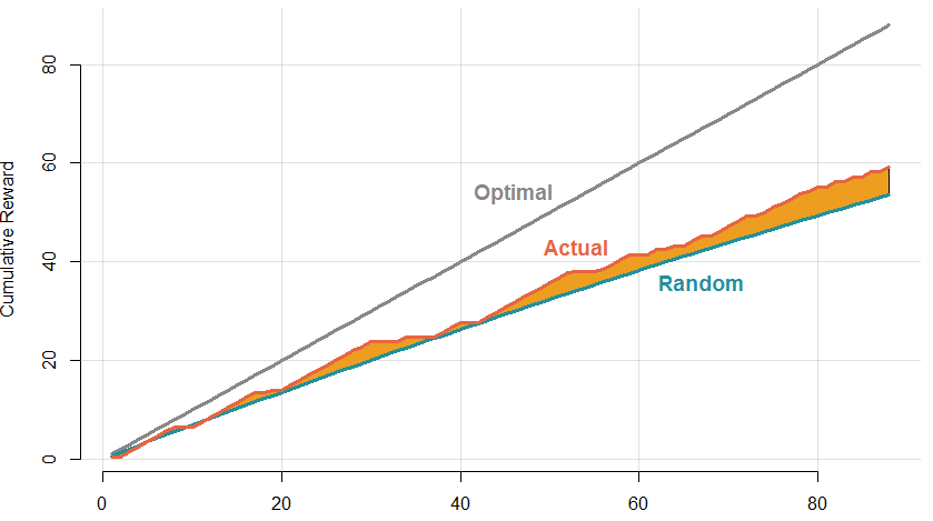
As you can see, Exp3 is consistently beating the random model. The margin is not amazing, but keep in mind that this is truly an adversarial problem where each trial increases the odds that subsequent trials with the same alternative will not pay off. Due to that, the random model would likely perform more poorly than estimated here.

The professional educational value of this method is debatable (I am not a teacher!), but I had some fun and I think my son and I both learned a lot.